
More Information
Submitted: December 15, 2025 | Accepted: December 27, 2025 | Published: December 29, 2025
Citation: Toufah A, Kadim MA, El Hafidi MY. Investigating Quantum Feature Maps in Quantum Support Vector Machines for Lung Cancer Classification. J Artif Intell Res Innov. 2025; 1(1): 100-110. Available from:
https://dx.doi.org/10.29328/journal.jairi.1001012
DOI: 10.29328/journal.jairi.1001012
Copyright license: © 2025 Toufah A, et al. This is an open access article distributed under the Creative Commons Attribution License, which permits unrestricted use, distribution, and reproduction in any medium, provided the original work is properly cited.
Keywords: Quantum machine learning; QSVM; Quantum feature maps; Lung cancer diagnosis; Paulifeaturemap; Healthcare AI

Investigating Quantum Feature Maps in Quantum Support Vector Machines for Lung Cancer Classification
A Toufah, MA Kadim and Moulay Youssef El Hafidi*
Quantum Physics and Spintronics Team, Condensed Matter Physics Laboratory (LPMC), Faculty of Sciences Ben M’Sik, Hassan II University of Casablanca, Morocco
*Corresponding author: Moulay Youssef El Hafidi, Quantum Physics and Spintronics Team, Condensed Matter Physics Laboratory (LPMC), Faculty of Sciences Ben M’Sik, Hassan II University of Casablanca, Morocco, Email: [email protected]
Background: Classical algorithms often struggle with the high dimensionality of medical data critical for early lung cancer diagnosis. While Quantum Machine Learning (QML) offers enhanced pattern recognition capabilities, the impact of specific quantum feature encoding strategies on diagnostic accuracy remains underexplored.
Methods: We evaluated Quantum Support Vector Machines (QSVM) using a dataset of 309 lung cancer patients, divided into six balanced subsets to mitigate class imbalance. Models were implemented on a qasm simulator, comparing three encoding strategies: ZFeatureMap, ZZFeatureMap, and PauliFeatureMap. Performance was assessed using standard classification metrics.
Results: The choice of feature map significantly influenced model efficacy. The PauliFeatureMap outperformed other kernels, achieving 100% classification accuracy in three of the six subsets, whereas ZFeatureMap and ZZFeatureMap yielded lower predictive consistency.
Conclusion: Quantum feature map selection is a decisive factor in QSVM performance. Specifically, the PauliFeatureMap demonstrates high separability for medical data, highlighting the potential of optimized quantum kernels to improve diagnostic precision.
Lung cancer remains one of the leading causes of cancer-related mortality worldwide, with early detection being critical to improving patient outcomes. Accurate and efficient diagnostic tools are therefore essential to assist healthcare professionals in making timely decisions. Machine learning (ML) techniques have demonstrated strong performance in various medical classification tasks, yet the complexity of biomedical data often challenges classical paradigms. This study explores the application of Quantum Machine Learning (QML) to address these challenges, specifically within the context of lung cancer diagnosis.
Background
Classically, Support Vector Machines (SVMs) operate by finding an optimal hyperplane that separates data points of different classes, relying on kernel functions to project data into higher-dimensional spaces [1]. While effective, classical models may struggle to capture the highly complex, non-linear data structures inherent in high-dimensional medical datasets.
Quantum computing offers a new framework for data processing by leveraging quantum mechanical principles such as superposition and entanglement [2]. Quantum Support Vector Machines (QSVMs) have been proposed as quantum-enhanced analogs of classical SVMs, aiming to exploit quantum feature spaces to achieve potentially superior classification capabilities [3]. A critical component in QSVMs is the feature map, which encodes classical data into quantum states. The design of these quantum feature maps determines how information is embedded into the quantum Hilbert space and can significantly influence the model’s ability to distinguish between classes [4].
Research questions
Despite the theoretical promise of QSVMs, the impact of specific quantum feature encoding strategies on diagnostic accuracy remains underexplored. The central research question of this study addresses this gap: How does the choice of quantum feature map affect the classification performance of QSVMs on real-world lung cancer data?
In this study, we investigate the role of different quantum feature maps in QSVM performance. We focus specifically on evaluating QSVMs utilizing three distinct encoding strategies, ZFeatureMap, ZZFeatureMap, and PauliFeatureMap, to assess how quantum data encoding impacts classification outcomes in a healthcare context.
Main contributions
This study advances the field of medical Quantum Machine Learning through the following contributions:
We provide a detailed comparative analysis of three quantum feature maps (Z, ZZ, and Pauli) to isolate the effect of entanglement and circuit depth on model performance.
Unlike many prior studies that rely on synthetic benchmarks, we validate these quantum methods on a real-world, balanced lung cancer dataset, demonstrating their practical applicability.
We identify the PauliFeatureMap as a superior encoding strategy for this specific medical task, achieving higher predictive consistency compared to simpler feature maps.
Related work
Support Vector Machines (SVMs) have been widely adopted in healthcare applications, particularly for disease diagnosis and classification tasks. In the context of cancer detection, SVM models have demonstrated robust performance due to their capacity to handle high-dimensional and complex data [5,6]. Several studies have reported high accuracy rates when applying SVMs to lung cancer datasets, establishing them as a reliable baseline method for clinical prediction tasks [7,8].
Quantum Machine Learning (QML) has recently begun to penetrate the healthcare domain. For example, Ramos-Calderer et al. applied quantum machine learning techniques to breast cancer classification tasks, showing the potential for quantum models to perform competitively with classical approaches [9]. Similarly, Schuld et al. explored circuit-centric quantum classifiers, highlighting the role of data encoding strategies in determining model performance [10].
A critical factor influencing QSVM performance is the selection of feature maps, which define how classical data is embedded into quantum Hilbert spaces. Studies such as Mitarai et al. [11] emphasize that appropriate feature mapping can significantly impact the classifier’s ability to separate classes in complex datasets. However, there remains a lack of systematic comparison of different quantum feature maps, especially in real-world medical datasets like lung cancer diagnosis.
This gap motivates the present study, where we conduct a comparative analysis of QSVM models utilizing various feature maps, applied to a lung cancer classification task. To clearly position our contributions within the existing landscape, Table 1 provides a comparative analysis of these related studies, highlighting the specific methodological gaps regarding feature map selection.
| Table 1: Comparative analysis of Classical and Quantum Machine Learning studies in medical diagnosis. | |||
| Reference | Methodology / Focus | Key Findings | Limitations / Research Gap |
| Asuntha et al. [5] | Classical SVM. Uses image processing (Gabor/Canny filters) and optimization (PSO, Genetic) for detection via CT, MRI, and Ultrasound images |
Achieved an accuracy of 89.5% for identifying cancerous nodules through feature extraction and selection | Relies entirely on classical computational paradigms and manual image feature extraction, potentially missing complex patterns in high-dimensional medical data |
| Schuld et al. [10] | Proposes low-depth variational algorithms using amplitude encoding for supervised learning. Tested on general UCI benchmarks like Breast. Cancer |
Achieved reasonable performance (e.g., 94.2% test accuracy on breast cancer) with significantly fewer parameters than classical neural networks | Focused on amplitude encoding and variational circuits rather than QSVM kernel methods. |
| Schuld & Killoran [20] | Explores implicit (kernel) and explicit (variational) approaches using squeezing feature maps in continuousvariable systems | Demonstrated that quantum feature maps can make data linearly separable in Fock space. | Focused primarily on theoretical foundations and low-dimensional synthetic benchmarks rather than high-dimensional clinical datasets. |
| A. Toufah et al. [24] | Compares classical SVM (RBF) with QSVM using a single feature map (ZZFeatureMap) on lung cancer patient subsets. |
QSVM demonstrated a marked improvement in recall (approx. 8% higher than classical SVM). | Utilized only one quantum encoding strategy (ZZFeatureMap); lacked a comparative analysis of how different feature map structures affect results. |
| Current Study |
Comparative study of Z, ZZ, and PauliFeatureMap encodings specifically for lung cancer classification. | PauliFeatureMap outperformed other kernels, achieving 100% accuracy in three subsets and a 96% average performance across all subsets. | – |
This section outlines the methodology used to classify lung cancer data with classical and quantum support vector machines (SVMs). We first describe the data preprocessing steps, followed by an overview of SVM and quantum SVM models. Finally, we present the evaluation metrics used to assess the models’ performance.
Dataset preprocessing and balancing
The dataset used in this study was retrieved from a public Kaggle repository [12]. It comprises 309 patient records, each annotated with a binary label indicating lung cancer diagnosis. The target variable, denoted by y∈ {0,1}, corresponds to whether a patient has lung cancer (1) or not (0). Among the 309 samples, 39 were labeled as negative cases (y = 0), while the remaining 270 samples were labeled as positive cases (y = 1).
The features in the dataset are primarily binary, encoded as Yes or No, except the gender variable (M or F) and age, which is continuous. To prepare the data for model training, all categorical binary features were numerically encoded using a simple mapping: Yes was mapped to 1, and No to 0. Similarly, gender was binarized by mapping M to 1 and F to 0. The continuous feature, age, was normalized using standardization:
(1)
Where x is the age value, µ is the sample mean, and σ is the sample standard deviation. This transformation ensures that age values have zero mean and unit variance, which improves numerical stability during training and is commonly used in machine learning [13].
No features were removed from the dataset. All variables were retained to preserve the original structure and maintain consistency across both classical and quantum models. Since the dataset was already clean and contained no missing values, no imputation or data cleaning procedures were required.
To address the issue of class imbalance, we constructed a set of six balanced subsets. Each subset includes all 39 negative samples and a unique, randomly selected set of 39 positive samples without replacement. Formally, let D = D0 ∪ D1, where D0 is the set of all samples such that y = 0 and 1 is the set where y = 1. We define each balanced subset Si as:
(2)
Where and , with . This subset design enables repeated evaluation of the models over different balanced configurations while avoiding data leakage and overlap. The choice of balancing method was guided by the desire to preserve data integrity while addressing class imbalance, which is crucial for accurate model performance in healthcare applications [14].
Support Vector Machine (SVM): Support Vector Machines (SVMs) are powerful supervised learning algorithms used for classification tasks, where the objective is to find a decision boundary that maximally separates data points belonging to different classes [15]. In the case of binary classification, given a training set , where xi ∈ Rd are the feature vectors and yi ∈ {−1,1} represent the class labels, the SVM learns a decision function of the form:
(3)
Here, w is the weight vector orthogonal to the decision hyperplane, and b is the bias term. The primary goal in SVM is to maximize the margin between the two classes, which is inversely proportional to the norm of the weight vector, i.e., . This process ensures that the decision boundary lies as far as possible from the closest data points, known as support vectors, minimizing the classification error.
However, in many real-world problems, data points from the two classes are not linearly separable in the original feature space. To handle such cases, the concept of soft-margin SVM is introduced. This formulation allows for misclassifications by introducing slack variables ξi ≥ 0, and the optimization problem becomes:
(4)
Subject to the constraints:
(5)
Where C is the regularization parameter that controls the trade-off between maximizing the margin and minimizing classification error. A larger C emphasizes minimizing misclassifications, while a smaller C favors larger margins with potential misclassifications.
To further extend SVM’s ability to handle non-linearly separable data, the kernel trick is introduced [16]. Instead of directly applying a non-linear transformation to the feature space, SVM computes the inner products of the transformed data points in a higher-dimensional space using a kernel function.
This allows the algorithm to implicitly map the data into a higher-dimensional space, where it might become linearly separable, without having to compute the transformation explicitly. The kernel function K(xi, xj) computes the inner product between two points xi and xj in the transformed feature space, thus enabling SVM to operate in this higher-dimensional space.
The most widely used kernel functions include the linear kernel, the polynomial kernel, and the radial basis function (RBF) kernel. The linear kernel, which is the simplest form of kernel, is defined as:
(6)
This kernel is particularly effective when the data is already linearly separable in the original feature space, as it does not perform any mapping but instead directly computes the inner product between the feature vectors.
In cases where the data exhibits non-linear relationships, the polynomial kernel is often used. This kernel maps the data into a higher-dimensional space where a polynomial decision boundary can separate the classes [17]. The polynomial kernel is given by:
(7)
Where c is a constant, and d is the degree of the polynomial. By adjusting the degree d, the polynomial kernel can represent different types of decision boundaries, from simple linear boundaries (when d = 1) to more complex, curved boundaries (as d increases).
The radial basis function (RBF) kernel, also known as the Gaussian kernel, is one of the most commonly used kernels due to its flexibility in capturing complex, non-linear relationships between data points [18]. The RBF kernel is defined as:
(8)
Where γ is a parameter that controls the spread of the Gaussian function. The RBF kernel’s ability to assign a higher weight to nearby data points and a lower weight to distant points makes it especially suitable for problems with complex decision boundaries. It is particularly effective when the data lies in a high-dimensional, non-linear feature space and can capture intricate relationships between the input features.
By using these kernel functions, SVM can classify data even in cases where the decision boundary is non-linear. The flexibility of the kernel trick is one of the reasons for SVM’s widespread success in various machine learning applications, including text classification, image recognition, and bioinformatics [19]. Moreover, the ability to tune parameters like C and γ allows the model to adapt to different types of data and classification tasks [18].
In this study, the RBF kernel was chosen due to its ability to handle non-linear data and the fact that no prior knowledge about the data distribution was available. The performance of the SVM was evaluated using various configurations of C and γ, optimizing these hyperparameters to achieve the best possible model performance.
An illustration of the SVM decision boundary with support vectors is shown in Figure 1, which visually depicts the decision hyperplane, margin boundaries, and support vectors in a two-dimensional space.
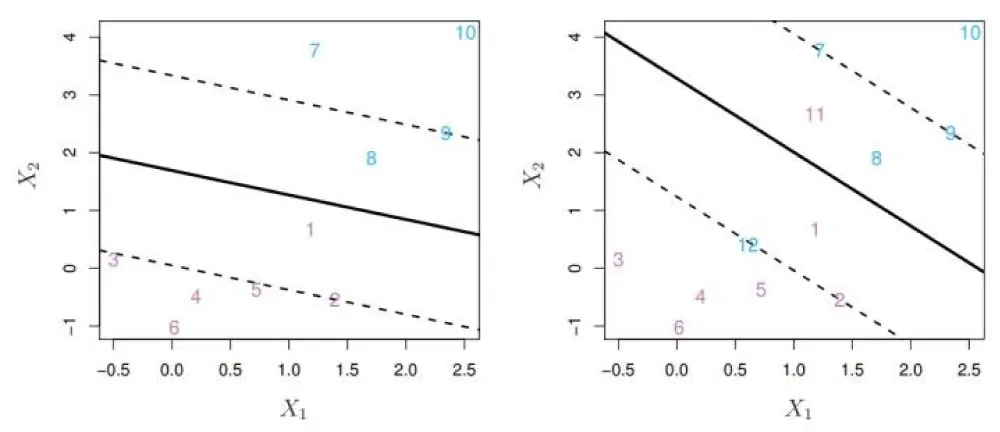
Figure 1: Illustration of a soft-margin SVM with support vectors, margin boundaries, and decision hyperplane.
Quantum Support Vector Machines
Quantum Support Vector Machines (QSVM) extend the classical SVM framework by leveraging the mathematical principles of quantum mechanics—particularly, quantum Hilbert spaces and state fidelity—to perform classification tasks. The key idea behind QSVM is to encode classical input data into quantum states and use quantum circuits to compute a kernel that captures similarities between these states.
In classical SVMs, the decision function depends on the computation of an inner product (or kernel) between input vectors. In QSVM, this inner product is replaced by the quantum fidelity between two quantum states:
(9)
where |ψ(x)> = Uϕ(x)|0>⟩⊗n is the quantum state representing the classical data point x, and Uϕ(x) is a data-encoding unitary circuit called the feature map.
This fidelity-based kernel is then used to construct the quantum kernel matrix, analogous to the classical kernel matrix. Once this matrix is computed—typically using the compute-uncompute method on a quantum simulator or device—the remainder of the QSVM pipeline proceeds classically, using a conventional optimization solver based on the dual formulation of the SVM problem:
(10)
Subject to
(11)
Where αi are the Lagrange multipliers, yi are the class labels, K(xi,xj) is the kernel function (quantum in the case of QSVM), and C is the regularization parameter.
QSVM thus blends quantum computation (for kernel evaluation) with classical optimization, aiming to exploit the expressive power of quantum states to better separate data in high-dimensional feature spaces.
Recent studies [20] have demonstrated that quantum kernels can outperform classical kernels on certain datasets by capturing richer structures through entanglement and interference. These theoretical advantages make QSVM a promising candidate for high-stakes classification tasks, such as in medical diagnostics.
Quantum feature maps: Quantum feature maps play a crucial role in Quantum Support Vector Machines (QSVM), as they define how classical data is embedded into quantum states. These feature maps influence the expressivity and noise sensitivity of the quantum model. In this subsection, we focus on three primary types of feature maps: ZFeatureMap, ZZFeatureMap, and PauliFeatureMap [21,22,23]. The quantum circuits corresponding to these feature maps are shown in Figures 2, 3, and 4, respectively.
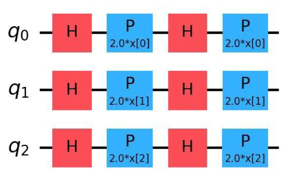
Figure 2: Quantum Circuit for ZFeatureMap.
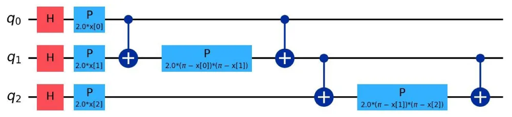
Figure 3: Quantum Circuit for ZZFeatureMap.
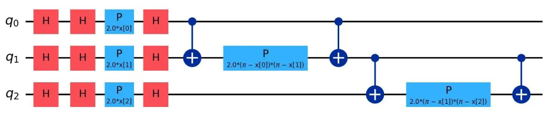
Figure 4: Quantum Circuit for PauliFeatureMap.
The ZFeatureMap is a Pauli-based feature map that applies single-qubit rotations around the Z-axis [24]. While it does not involve entanglement, which limits its capacity to capture feature correlations, it is simple and efficient to implement, making it well-suited for datasets where features are assumed to be uncorrelated.
Though the theoretical formulation of the ZFeatureMap includes only Rz(2xk) operations, in practice, it is often preceded by Hadamard gates on each qubit to enhance the expressivity of the state. The unitary encoding is given by:
(12)
where xk is the k-th classical input, and Zk is the Pauli-Z operator acting on the k-th qubit.
The ZZFeatureMap introduces pairwise interactions between qubits using entanglement through the operation. It is better suited for correlated data and has higher expressive capacity than the ZFeatureMap, but is more sensitive to quantum noise. The theoretical formulation is:
(13)
This entanglement allows the feature map to encode second-order feature interactions, which are crucial for tasks such as cancer diagnosis and fraud detection.
The PauliFeatureMap encodes classical data using rotations around all three Pauli axes (X, Y, Z) and includes entanglement terms. It is defined as:
(14)
This map is the most expressive but also the most susceptible to noise due to the use of gates that flip the computational basis states, such as X and Y.
The choice of an appropriate feature map depends on two major factors: the nature of the data and the noise resilience of the quantum device.
- Thermal Relaxation Noise: ZFeatureMap is relatively resistant but can suffer from phase loss. ZZFeatureMap is more sensitive due to entanglement. PauliFeatureMap is highly sensitive to bit-flip noise introduced by X and Y gates.
- Data Type: ZFeatureMap is best for uncorrelated features and benefits from rapid execution. ZZFeatureMap is ideal for pairwise correlated features, albeit with a higher computational cost. PauliFeatureMap, while powerful, requires careful noise mitigation strategies due to its complexity.
Statistical Analysis and Parameter Tuning
To ensure the reproducibility and robustness of our classification results, we implemented a systematic hyperparameter optimization strategy. For the classical SVM models, we utilized a **Grid Search** approach. The regularization parameter C, which controls the trade-off between margin maximization and classification error, was optimized within the search space C∈ {0.1,1,10,100}. For the RBF kernel, the kernel coefficient γ was simultaneously optimized within the range γ∈ {0.001,0.01,0.1,1}.
For the Quantum Support Vector Machine (QSVM), the quantum kernel matrices were precomputed using the Qasm simulator backend from the Qiskit framework. These precomputed kernels were then integrated into the classical SVM optimization pipeline using the scikit-learn library. To validate the statistical significance of our findings and mitigate the bias often introduced by class imbalance, we performed independent evaluations on the six balanced subsets defined in Section 3.1. The final performance metrics reported (Accuracy, Precision, Recall, Specificity, F1-Score) represent the aggregated average across these independent trials, ensuring that the observed performance gains are consistent and not artifacts of a specific random sampling.
Evaluation metrics
In this study, several key performance metrics were used to evaluate the effectiveness of the classification models, namely accuracy, precision, recall, specificity, and F1-score. These metrics provide a comprehensive understanding of how well the models perform in distinguishing between the two classes, which is especially important in healthcare applications where a correct classification is critical.
Accuracy is one of the most straightforward evaluation metrics, defined as the ratio of correctly classified instances to the total number of instances. It is given by:
Where:
- True Positives are the number of instances correctly classified as positive.
- True Negatives are the number of instances correctly classified as negative.
- False Positives are the number of instances incorrectly classified as positive.
- False Negatives are the number of instances incorrectly classified as negative.
While accuracy is useful in many cases, it can be misleading when dealing with imbalanced datasets, which is why additional metrics are often considered.
Precision evaluates the number of positive predictions made by the model that are actually correct. It is defined as:
Precision is particularly important when the cost of a false positive is high. In medical applications, a false positive might result in unnecessary treatment, so maximizing precision is crucial.
Recall, also known as sensitivity or the true positive rate, measures the ability of the model to identify positive instances correctly. It is given by:
In the context of healthcare, recall is especially important because it indicates how well the model can identify true positive cases (e.g., identifying patients who are at risk of developing a certain disease).
A higher recall means fewer false negatives, which is critical when missing a positive case could have severe consequences.
Specificity, or the true negative rate, measures the proportion of negative instances that are correctly identified. It is defined as:
This metric is particularly useful when the cost of a false positive is high, as it measures how well the model avoids incorrectly labeling negative instances as positive.
F1-score is the harmonic mean of precision and recall, providing a balance between the two. It is particularly useful when both false positives and false negatives carry similar importance. It is defined as:
The F1-score is a crucial metric when the class distribution is imbalanced, as it provides a better measure of the model’s performance in both identifying positive and negative instances.
These evaluation metrics provide a comprehensive assessment of the model’s performance and are particularly important in imbalanced datasets where accuracy alone might not be sufficient. Each metric captures a different aspect of the classification process, helping to ensure that the models perform well in detecting both positive and negative instances in the data [25,26].
The experimental setup for this study was based on a publicly available lung cancer dataset retrieved from Kaggle [12]. This dataset consists of 309 patient records, each annotated with a binary label indicating the presence (1) or absence (0) of lung cancer. Among the collected samples, 270 correspond to positive cases and 39 to negative cases, highlighting a significant class imbalance. The features are primarily binary (Yes/No responses), except for the gender attribute (Male/Female) and age, which is a continuous variable. All binary categorical features were numerically encoded by mapping ”Yes” to 1 and ”No” to 0, while gender was encoded by mapping ”M” to 1 and ”F” to 0. The continuous age feature was standardized using z-score normalization, ensuring zero mean and unit variance, a common practice to enhance numerical stability during model training [27]. No features were discarded from the original dataset to maintain a consistent feature space across classical and quantum models. Additionally, the dataset exhibited no missing values, eliminating the need for imputation or further cleaning procedures. To address the substantial class imbalance, six balanced subsets were constructed. Each subset contains all 39 negative samples and 39 unique positive samples selected randomly without replacement, as summarized in Table 2. This strategy ensures that model evaluation is performed over multiple balanced configurations without overlap, preserving data integrity and minimizing bias—a critical consideration in healthcare-related machine learning tasks [28].
| : Summary of the lung cancer dataset used in this study. | |
| Characteristic | Details |
| Total Samples | 309 |
| Positive Cases (y = 1) | 270 |
| Negative Cases (y = 0) | 39 |
| Number of Features | 15 (14 binary, 1 continuous) |
| Missing Values | None |
| Data Balancing Strategy | 6 balanced subsets (every 78 samples) |
| FFeature Encoding | Primary mapping, Gender mapping, Age standardization |
To better understand the structure and variability of the data within each balanced subset, a Principal Component Analysis (PCA) [29] was performed. PCA is widely used for dimensionality reduction and visualization in machine learning, enabling the projection of high-dimensional data into two principal components while preserving as much variance as possible [30]. Figure 5 illustrates the two-dimensional PCA projections for each of the six subsets. Each plot displays the separation between positive and negative classes, providing a visual confirmation that, despite balancing, some overlap remains between classes. Such overlaps emphasize the classification challenge and justify the need for sophisticated modeling approaches like quantum-enhanced classifiers.
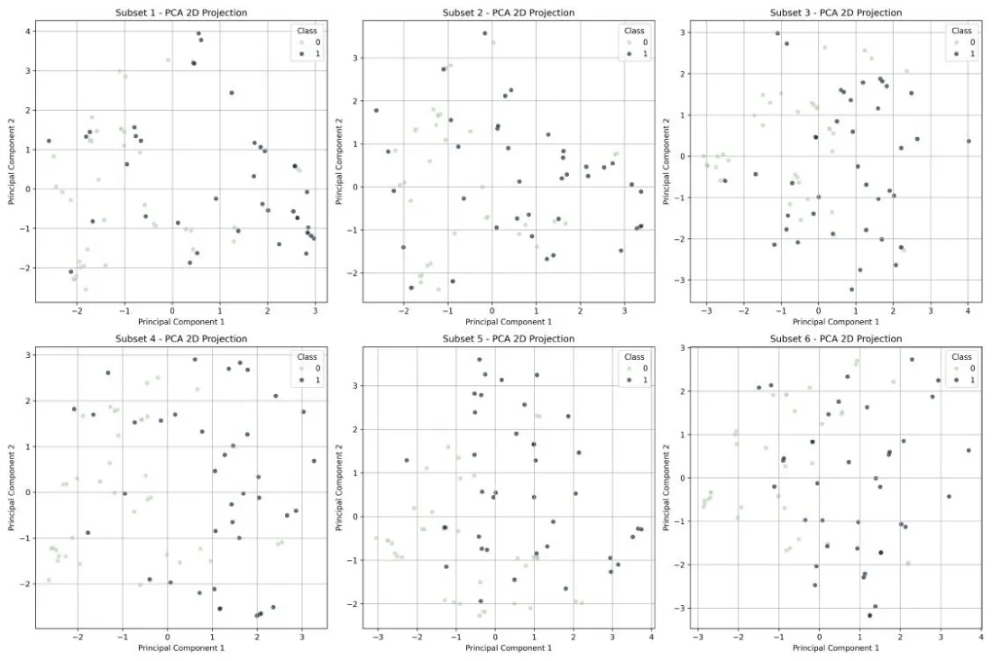
Figure 5: PCA visualization of the six balanced subsets. Each plot represents a two-dimensional projection of the samples, colored by class label..
In order to establish a baseline for evaluating quantum models, we first conducted a comparative analysis between classical Support Vector Machines (SVMs) and Quantum Support Vector Machines (QSVMs). For the classical SVM models, three different kernel functions were tested: linear, polynomial, and radial basis function (RBF). The evaluation was performed across the six balanced subsets described previously, and the results were averaged to ensure robustness. The performance metrics considered include accuracy, precision, recall, specificity, and F1-score, which provide a comprehensive view of the classification effectiveness. For the linear kernel, SVM achieved an accuracy of 0.91, precision of 0.93, recall of 0.90, specificity of 0.92, and F1-score of 0.90. For the polynomial kernel, the results improved with an accuracy of 0.94, precision of 0.98, recall of 0.90, specificity of 0.98, and F1-score of 0.93. The radial basis function (RBF) kernel provided the best results, with an accuracy of 0.95, precision of 0.98, recall of 0.92, specificity of 0.98, and F1-score of 0.95.
For the quantum approach, QSVM models were trained using three different quantum feature maps: ZFeatureMap, ZZFeatureMap, and PauliFeatureMap. The PauliFeatureMap was configured with Pauli rotations on the Z, X, and Y axes, enabling the encoding of complex feature correlations. Each quantum model was evaluated on the same six balanced subsets to ensure a fair comparison with its classical counterpart. The results for these feature maps are summarized as follows: for ZFeatureMap, the model achieved an accuracy of 0.88, precision of 0.95, recall of 0.81, specificity of 0.94, and F1-score of 0.86; for ZZFeatureMap, the results were an accuracy of 0.91, precision of 0.87, recall of 0.96, specificity of 0.85, and F1-score of 0.91; and for PauliFeatureMap, the model achieved a consistent performance of 0.96 across all metrics, including accuracy, precision, recall, specificity, and F1-score.
The comparative results are summarized in two grouped bar charts. The first chart presents the average performance of classical SVM models across the different kernel types, while the second chart illustrates the average performance of QSVM models across the three feature maps. Figures 6 and 7 provide a visual summary of these findings, highlighting the variations in model behavior depending on the choice of kernel or quantum feature map.
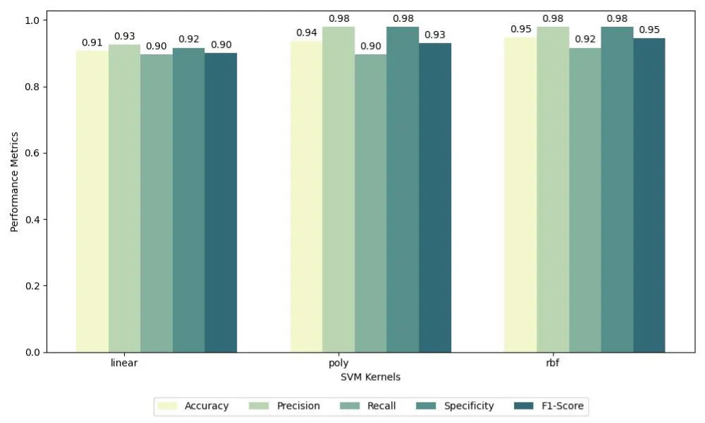
Figure 6: Grouped bar chart showing the average performance metrics of SVM models across different kernels (linear, polynomial, RBF) over six balanced subsets..
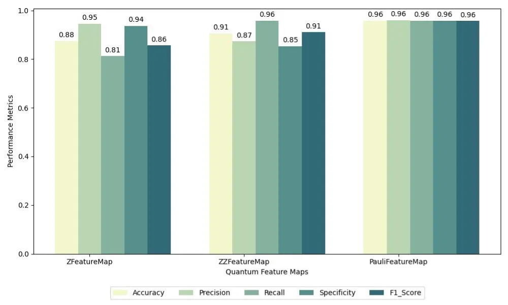
Figure 7: Grouped bar chart showing the average performance metrics of QSVM models across different quantum feature maps (ZFeatureMap, ZZFeatureMap, PauliFeatureMap with Z, X, and Y rotations) over six balanced subsets.
Building upon the preliminary comparison between classical SVM and Quantum Support Vector Machine (QSVM), we now shift our attention to a more in-depth analysis of QSVM’s performance across
The six balanced subsets. In this section, we focus specifically on the impact of different quantum feature maps—namely, ZFeatureMap, ZZFeatureMap, and PauliFeatureMap—on QSVM’s ability to classify the lung cancer dataset. The performance of QSVM is evaluated using five key metrics: accuracy, precision, recall, specificity, and F1-score, all of which are presented in Table 3.
| Table 3: Performance of QSVM across the 6 balanced subsets using three different quantum feature maps: ZFeatureMap, ZZFeatureMap, and PauliFeatureMap. The metrics shown include accuracy, precision, recall, specificity, and F1-score for each subset under the corresponding feature map. | ||||||
| Feature Map | Subset | Accuracy | Precision | Recall | Specificity | F1-Score |
| ZFeatureMap | 1 2 3 4 5 6 |
0.875 0.875 0.875 0.875 1.000 0.750 |
0.875 1.000 0.800 1.000 1.000 1.000 |
0.875 0.750 1.000 0.750 1.000 0.500 |
0.875 1.000 0.750 1.000 1.000 1.000 |
0.875 0.857 0.889 0.857 1.000 0.667 |
| ZZFeatureMap | 1 2 3 4 5 6 |
1.000 0.875 0.875 0.937 0.875 0.875 |
1.000 0.875 0.8000 0.889 0.800 0.875 |
1.000 0.875 1.000 1.000 1.000 0.875 |
1.000 0.875 0.750 0.875 0.750 0.875 |
1.000 0.875 0.889 0.941 0.889 0.875 |
| PauliFeatureMap | 1 2 3 4 5 6 |
0.875 0.937 0.937 1.000 1.000 1.000 |
0.875 1.000 0.889 1.000 1.000 1.000 |
0.875 0.875 1.000 1.000 1.000 1.000 |
0.875 1.000 0.875 1.000 1.000 1.000 |
0.875 0.933 0.941 1.000 1.000 1.000 |
The results provide insight into how each feature map influences the overall classification performance of QSVM. The three feature maps represent different quantum encoding schemes, each of which can capture and utilize the data’s quantum characteristics in distinct ways. As detailed in the following table, we compare the performance of QSVM models across the six subsets, with each subset being evaluated using the three feature maps.
From the results shown in Table 3, we observe that the PauliFeatureMap consistently yields the highest performance across all subsets, achieving perfect scores in Subsets 4, 5, and 6. This suggests that PauliFeatureMap is particularly effective at capturing the complex feature relationships required for accurate classification, leading to perfect recall, precision, and F1-score in these subsets.
The ZZFeatureMap, while demonstrating solid performance, shows some variability in its results. It achieves perfect scores for Subset 1, Subset 5, and Subset 6, but in other subsets, its performance drops slightly, particularly in recall. This variability indicates that while ZZFeatureMap is effective, its performance can be sensitive to the characteristics of the data in each subset.
The ZFeatureMap also performs well but generally yields lower results in comparison to the other two feature maps. It is most consistent in terms of performance, achieving stable accuracy across the subsets, but its recall and precision tend to be lower, especially in Subsets 2, 3, and 6. This suggests that ZFeatureMap may not be as well-suited to capturing complex patterns in the data compared to ZZFeatureMap and PauliFeatureMap.
Overall, these results demonstrate the importance of selecting the right feature map for quantum machine learning tasks. The PauliFeatureMap appears to be the most effective feature map for this task, particularly in subsets where the data may involve more complex relationships between the features. However, the ZZFeatureMap and ZFeatureMap also show promise, with ZZFeatureMap achieving strong results in several subsets. The choice of feature map plays a crucial role in the QSVM’s classification performance, and further experiments could explore whether additional feature maps could lead to even better results.
In this study, we examined the role of quantum feature maps, ZFeatureMap, ZZFeatureMap, and PauliFeatureMap, in Quantum Support Vector Machines (QSVM), particularly focusing on their structural differences, susceptibility to quantum noise, and data suitability.
Each feature map presents a trade-off between circuit complexity, expressivity, and robustness to quantum decoherence. The ZFeatureMap applies only single-qubit Z-rotations, resulting in shallow circuits with no entanglement. This simplicity makes it less sensitive to hardware noise and faster to execute, which is beneficial in near-term quantum devices. However, due to the absence of entanglement, it is best suited for datasets with uncorrelated features. Moreover, it begins to lose phase coherence under thermal relaxation, which causes high-probability states to degrade, thereby affecting classification performance in more complex tasks.
The ZZFeatureMap builds upon the ZFeatureMap by adding pairwise entanglement through controlledZZ interactions. This structure enables it to capture dependencies between features, making it more appropriate for datasets with pairwise correlations. As a result, it tends to achieve better classification accuracy than the ZFeatureMap when feature interactions are significant. Nevertheless, the entanglement increases the circuit depth and sensitivity to thermal noise. Thermal relaxation in ZZFeatureMap not only causes phase decay as seen in the ZFeatureMap but also amplifies the effect due to entanglement, leading to higher degradation in quantum state fidelity.
The PauliFeatureMap generalizes feature encoding further by using a combination of Pauli gates (X, Y, Z), introducing both expressivity and complexity. Unlike the ZZFeatureMap, it often avoids entanglement but uses basis-changing operations that make it highly sensitive to bit-flip errors. This sensitivity arises because X and Y gates alter the computational basis, potentially leading to the emergence of new, unlikely states under thermal noise. While powerful in capturing intricate data patterns in simulations, the PauliFeatureMap shows higher variance in performance and may not generalize well on noisy intermediate-scale quantum (NISQ) hardware. Notably, it is still better suited for uncorrelated datasets and offers fast implementation due to limited entanglement, albeit with deeper single-qubit operations.
To contextualize the improvements achieved by our proposed approach, we compared our results against relevant state-of-the-art methods in both classical and quantum domains.
In the classical domain, Asuntha et al. (2016) utilized classical SVMs with optimized feature extraction techniques (Gabor and Canny filters) for lung cancer detection, achieving an accuracy of 89.5%. In contrast, our QSVM model utilizing the PauliFeatureMap demonstrated significantly higher predictive consistency, achieving a perfect accuracy of 100% in three balanced subsets and maintaining a 96% average across all trials. This suggests that projecting data into quantum Hilbert spaces can reveal separation hyperplanes that classical feature extraction may miss.
Regarding quantum benchmarks, our results surpass those reported in early variational studies. For instance, Schuld et al. (2018) reported a test accuracy of 94.2% on breast cancer datasets using circuit-centric variational classifiers. While their work utilized amplitude encoding to reduce parameter count, our kernel-based approach with Pauli encodings yielded superior accuracy on the lung cancer dataset. Furthermore, while Schuld and Killoran (2018) established the theoretical foundation that quantum feature maps can make data linearly separable in Fock space using synthetic benchmarks (circles, moons), our study validates this theory on high-dimensional clinical data. We demonstrate that the theoretical advantage of quantum feature spaces translates into tangible diagnostic improvements in a real-world healthcare context.
In summary, our results suggest that:
- ZFeatureMap is most resilient to hardware noise and suitable for simpler, uncorrelated data, though limited in capturing complex relationships.
- ZZFeatureMap strikes a balance between expressivity and practicality, being ideal for correlated data but moderately affected by noise due to entanglement.
- PauliFeatureMap is the most expressive in theory and practice, outperforming state-of-the-art benchmarks with 96% average accuracy, though it requires careful handling of bit-flip noise due to basis-altering operations.
Choosing an appropriate feature map must account for both the nature of the dataset and the physical limitations of the quantum device. Future work may explore adaptive feature maps or hybrid classical-quantum encodings that better leverage the benefits of each approach while minimizing their drawbacks.
This research explored the impact of quantum feature map design on the performance of Quantum Support Vector Machines (QSVM) in binary classification tasks. By focusing on three commonly used feature maps—ZFeatureMap, ZZFeatureMap, and PauliFeatureMap—we demonstrated how each architecture uniquely influences model behavior in terms of expressivity, noise resilience, and data suitability. Our findings revealed that the ZFeatureMap is well-suited for uncorrelated datasets due to its simple structure and reduced sensitivity to noise, though it may suffer from phase relaxation. The ZZFeatureMap, incorporating quantum entanglement, showed improved performance on correlated data but exhibited increased vulnerability to thermal relaxation errors due to its deeper circuit. In contrast, the PauliFeatureMap, while theoretically more expressive, was most affected by noise—particularly bitflip errors—because of its use of non-diagonal gates that alter the computational basis. These results highlight the critical role of feature map selection in optimizing QSVM performance and emphasize the importance of aligning quantum circuit design with both data structure and hardware limitations for practical quantum machine learning applications.
Declarations
Availability of data and materials: The dataset used in this study is publicly available on Kaggle at the following link: https://www.kaggle.com/datasets/ahmetsendil/lung-cancer-dataset
Author contributions
Moulay Youssef El Hafidi contributed to the conceptualization, methodology, supervision, and validation of the study. Mohamed Achraf Kadim was responsible for the theoretical modeling and formal analysis. Achraf Toufah prepared the dataset, implemented the quantum circuits, carried out the coding and simulations, and drafted the manuscript. All authors read and approved the final manuscript.
Funding
This research received no specific grant from any funding agency in the public, commercial, or not-for-profit sectors.
Competing interests: The authors declare that they have no competing interests.
- Cristianini N, Shawe-Taylor J. An introduction to support vector machines and other kernel-based learning methods. Cambridge (UK): Cambridge University Press; 2000. Available from: https://www.cambridge.org/core/books/an-introduction-to-support-vector-machines-and-other-kernelbased-learning-methods/A6A6F4084056A4B23F88648DDBFDD6FC
- Schuld M, Sinayskiy I, Petruccione F. An introduction to quantum machine learning. Contemp Phys. 2015;56(2):172–185. Available from: https://doi.org/10.1080/00107514.2014.964942
- Havlíček V, Córcoles AD, Temme K, Harrow AW, Kandala A, Chow JM, Gambetta JM. Supervised learning with quantum-enhanced feature spaces. Nature. 2019;567:209–212. Available from: https://doi.org/10.1038/s41586-019-0980-2
- Biamonte J, Wittek P, Pancotti N, Rebentrost P, Wiebe N, Lloyd S. Quantum machine learning. Nature. 2017;549:195–202. Available from: https://doi.org/10.1038/nature23474
- Asuntha A, Brindha SI, Srinivasan A. Lung cancer detection using SVM algorithm and optimization techniques. J Chem Pharm Sci. 2016;9(4):3198–3203. Available from: https://www.jchps.com/issues/Volume%209_Issue%204/jchps%209(4)%20286%200450716%203198-3203.pdf
- Zhao W, Davis CE. A modified artificial immune system-based pattern recognition approach—An application to clinical diagnostics. Artif Intell Med. 2011;52(1):1–9. Available from: https://doi.org/10.1016/j.artmed.2011.03.001
- Alam J, Alam S, Hossan A. Multi-stage lung cancer detection and prediction using multi-class SVM classification. In: Proceedings of the IEEE International Conference on Computer, Communication, Chemical, Materials and Electronic Engineering (IC4ME2); 2018. p. 1–4. Available from: https://doi.org/10.1109/IC4ME2.2018.8465593
- Parveen SS, Kavitha C. Classification of lung cancer nodules using SVM kernels. Int J Comput Appl. 2014;95(25):25–28. Available from: https://www.ijcaonline.org/archives/volume95/number25/16751-7013/
- Kaveh S, Arezi E, Khedri Z, Sohrabei S. Investigating the application of quantum machine learning in breast cancer: a systematic review. Arch Breast Cancer. 2025;12:130–142. Available from: https://doi.org/10.32768/abc.2025122130-142
- Schuld M, Bocharov A, Svore KM, Wiebe N. Circuit-centric quantum classifiers. Phys Rev A. 2020;101:032308. Available from: https://doi.org/10.1103/PhysRevA.101.032308
- Mitarai K, Negoro M, Kitagawa M, Fujii K. Quantum circuit learning. Phys Rev A. 2018;98:032309. Available from: https://doi.org/10.1103/PhysRevA.98.032309
- Şendil A. Lung cancer dataset [Internet]. Kaggle; 2025 [cited 2025 Dec 25]. Available from: https://www.kaggle.com/datasets/ahmetsendil/lung-cancer-dataset
- Oyelade J, Isewon I, Oladipupo O, Emebo O, Omogbadegun Z, Aromolaran O, Uwoghiren E, Olaniyan D, Olawole O. Data clustering: algorithms and their applications. In: Proceedings of the IEEE International Conference on Computer Science and Its Applications (ICCSA); 2019. p. 71–81. Available from: https://doi.org/10.1109/ICCSA.2019.000-1
- Chawla NV, Bowyer KW, Hall LO, Kegelmeyer WP. SMOTE: synthetic minority over-sampling technique. J Artif Intell Res. 2002;16:321–357. https://doi.org/10.1613/jair.953
- Boser BE, Guyon IM, Vapnik VN. A training algorithm for optimal margin classifiers. In: Proceedings of the Fifth Annual Workshop on Computational Learning Theory (COLT ’92); 1992. https://doi.org/10.1145/130385.130401
- Combarro E, González-Castillo S. A practical guide to quantum machine learning and quantum optimization: hands-on approach to modern quantum algorithms. 2023. Available from: https://quantumatlas.ir/wp-content/uploads/2025/01/A-Practival-Guide-to-Quantum-Machine-Learning-and-Quantum-Optimization.pdf
- Pontil M, Verri A. Support vector machines for 3D object recognition. IEEE Trans Pattern Anal Mach Intell. 1998;20(6):637–646. Available from: https://doi.org/10.1109/34.683777
- Schölkopf B, Smola AJ. Learning with kernels. Cambridge (MA): MIT Press; 2001. https://doi.org/10.7551/mitpress/4175.001.0001
- Cortes C, Vapnik V. Support-vector networks. Mach Learn. 1995;20:273–297. Available from: https://doi.org/10.1007/BF00994018
- Schuld M, Killoran N. Quantum machine learning in feature Hilbert spaces. Phys Rev Lett. 2019;122:040504. Available from: https://doi.org/10.1103/PhysRevLett.122.040504
- Suzuki T, Hasebe T, Miyazaki T. Quantum support vector machines for classification and regression on a trapped-ion quantum computer. Quantum Mach Intell. 2024;6. Available from: https://doi.org/10.1007/s42484-024-00165-0
- Özpolat Z, Yıldırım Ö, Karabatak M. The effect of linear discriminant analysis and quantum feature maps on QSVM performance for obesity diagnosis. Balkan J Electr Comput Eng. 2024. Available from: https://doi.org/10.17694/bajece.1475896
- Bartkiewicz K, Gneiting C, Černoch A, Jiráková K, Lemr K, Nori F. Experimental kernel-based quantum machine learning in finite feature space. Sci Rep. 2020;10:12356. Available from: https://doi.org/10.1038/s41598-020-68911-5
- Toufah MA, Kadim MA, El Hafidi MY. Overcoming SVM limitations in lung cancer classification with a quantum feature map. BMC Artif Intell. 2025;1. Available from: https://doi.org/10.1186/s44398-025-00016-3
- Kim H, Seo J. High-performance FAQ retrieval using an automatic clustering method of query logs. Inf Process Manag. 2006;42(3):650–661. Available from: https://doi.org/10.1016/j.ipm.2005.04.002
- Powers DMW. Evaluation: from precision, recall and F-measure to ROC, informedness, markedness and correlation. arXiv. 2020:2010.16061. Available from: https://arxiv.org/abs/2010.16061
- Huang L. Normalization techniques in deep learning. San Rafael (CA): Morgan & Claypool Publishers; 2022. https://doi.org/10.1007/978-3-031-14595-7
- Salmi M, Atif D, Oliva D, Abraham A, Ventura S. Handling imbalanced medical datasets: review of a decade of research. Artif Intell Rev. 2024;57. Available from: https://doi.org/10.1007/s10462-024-10884-2
- Jolliffe IT. Principal component analysis. New York: Springer-Verlag; 2002. Available from: https://doi.org/10.1007/b98835